
How the Arm’s Length Range Is Actually Calculated Under Rule 10CA: A Worked Example
CA Mithilesh Reddy
20 Oct 2026 · 5 min read
On this page
Note: the dataset and margin figures used below are illustrative, invented for explanatory purposes only, and do not represent any real company or filed study.
Direct answer
Under Rule 10CA of the Income-tax Rules, where a comparable dataset has six or more entries, the arm’s length range is constructed by sorting the margins in ascending order and computing the 35th and 65th percentile points of that ordered dataset. If the tested party’s actual result falls inside that range, it is deemed arm’s length; if it falls outside, the arm’s length price is taken as the dataset’s median rather than the nearer edge of the range. This article walks through that calculation with an illustrative nine-company dataset, including the percentile interpolation step and the tolerance-band check most manual spreadsheet models get subtly wrong.
What this guide covers
Most explanations of Indian transfer pricing benchmarking stop at the phrase “35th to 65th percentile” without showing the arithmetic behind it, which leaves a real gap for anyone trying to sanity-check a benchmarking report or build their own working file. This article fills that gap with a full worked example, referencing Rule 10CA and Section 92C of the Income-tax Act directly, and notes where the same substantive mechanics are being recodified under the Income-tax Act, 2025, which took effect 1 April 2026.
Step one: build the ordered dataset
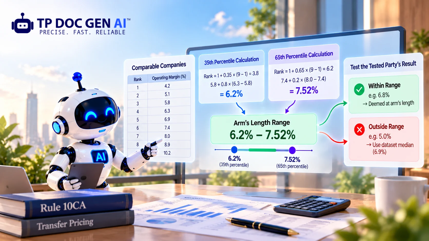
Suppose a benchmarking search for a routine service provider has produced nine comparable companies, each with an operating margin (operating profit over operating cost) for the relevant financial year. Sorted ascending, the illustrative dataset is: 4.2%, 5.1%, 5.8%, 6.3%, 6.9%, 7.4%, 8.0%, 8.9%, 10.2%. With nine entries, this dataset clears the six-or-more threshold at which Rule 10CA(4) requires a range rather than a simple arithmetical mean.
Step two: locate the 35th and 65th percentile points
Percentile calculation on a small dataset requires interpolation between the two nearest ranked values, not simply picking the nearest entry. Using linear interpolation - the method most spreadsheet formulas and statistical software default to - the rank position for a given percentile p in a dataset of n entries is 1 + p × (n − 1). For the 35th percentile: 1 + 0.35 × 8 = 3.8, meaning the value sits 80% of the way between the third ranked value (5.8%) and the fourth (6.3%), giving 5.8 + 0.8 × (6.3 − 5.8) = 6.2%. For the 65th percentile: 1 + 0.65 × 8 = 6.2, meaning the value sits 20% of the way between the sixth ranked value (7.4%) and the seventh (8.0%), giving 7.4 + 0.2 × (8.0 − 7.4) = 7.52%. The arm’s length range for this illustrative dataset is therefore approximately 6.2% to 7.52%.
Step three: test the tested party’s actual result against the range
If the tested party’s actual operating margin for the year is, say, 6.8%, it falls inside the 6.2%–7.52% range, and under Rule 10CA(5) the transaction is deemed to be at arm’s length with no further adjustment required. If instead the tested party’s actual margin is 5.0%, it falls outside the range, and Rule 10CA(6) directs that the arm’s length price be taken as the dataset’s median - here, the fifth ranked value of the nine, or 6.9% - rather than adjusted only to the nearer edge of the range at 6.2%. This distinction matters in practice: a common error is assuming an out-of-range result is corrected to the closest boundary of the range, when the rule in fact directs a correction to the median, which can be a materially larger adjustment.
Step four: the tolerance-band conversion most spreadsheets get wrong
Where a dataset has fewer than six entries and the arithmetical mean applies under Rule 10CA(7), a further test applies: if the variation between the arm’s length price and the actual transaction price does not exceed the tolerance percentage the Central Board of Direct Taxes notifies annually - 3% in most cases, notified periodically in the Official Gazette - the actual transaction price is still deemed arm’s length despite technically sitting outside the calculated figure. The step that trips up manual models is that this tolerance test operates on the transaction’s absolute price or value, not directly on a margin percentage - so a benchmarking exercise conducted in margin-percentage terms has to convert back to the underlying transaction value before the tolerance check can be applied correctly. A spreadsheet that never performs this conversion, and instead checks whether the margin percentages themselves sit within 3 percentage points of each other, is testing something Rule 10CA does not actually say.
What a reviewer should independently re-check, not just accept
A second reviewer checking a benchmarking file is not adding value by re-reading the final range and confirming it looks reasonable - a plausible-looking wrong number looks exactly as reasonable as a correct one. A genuinely useful review re-performs the specific mechanical steps above independently: reordering the dataset from the raw comparable figures rather than trusting the file’s stated ordering, recalculating the percentile position using the same interpolation method the file claims to use, and confirming that an out-of-range case was actually adjusted to the median rather than the nearer boundary. This is a materially different, more time-consuming check than reading a finished report for internal consistency, and it is precisely the check a Transfer Pricing Officer is trained to perform during a scrutiny assessment - which means a reviewer who has not already performed it internally is finding out for the first time, during an actual dispute, whether the file’s arithmetic holds up.
Why practitioners should understand the manual mechanics even when using software
There is a reasonable question of whether any of this matters once a platform is performing the calculation automatically and correctly - and the answer is that understanding the underlying mechanics remains necessary for exactly the reason a pilot still needs to understand aerodynamics despite flying an aircraft with automated controls. A practitioner who understands why the median substitution rule exists, and why the tolerance test operates on transaction value rather than margin percentage, is equipped to explain the resulting figure to a client, to a Transfer Pricing Officer, or to a Dispute Resolution Panel in terms that demonstrate genuine command of the methodology - rather than being able to state only that “the software calculated it this way” when asked to justify a specific figure. Automation should remove the risk of manual arithmetic error, not the practitioner’s own understanding of what the arithmetic is actually doing and why.
Why this level of mechanical detail is not a formality
The gap between “the range is 35th to 65th percentile” as a description and the actual interpolation, median-substitution and tolerance-conversion steps above is exactly where a manually built spreadsheet model most often diverges from what a Transfer Pricing Officer’s own calculation produces - not through a dramatic error, but through a percentile method that rounds instead of interpolates, or a median substitution rule that is coded as “nearest boundary” instead of “dataset median,” or a tolerance check applied in the wrong unit. Each of these produces a plausible-looking, wrong number, and because the error sits inside a formula rather than in a reviewable narrative, it is one of the hardest mistakes in a transfer pricing file to catch by inspection alone.
What changes with an even-numbered dataset
The illustrative example above uses nine comparables specifically because an odd-numbered dataset makes the median straightforward to identify - it is simply the middle ranked value. With an even-numbered dataset, the median is itself an interpolation: the average of the two middle ranked values, rather than a single observed data point. Consider a ten-company version of the same dataset, adding a tenth comparable at 11.0% to the nine used above. The median is now the average of the fifth and sixth ranked values - 6.9% and 7.4% - giving a median of 7.15%, a figure that does not correspond to any single comparable’s actual reported margin. This distinction matters specifically because Rule 10CA(6) directs an out-of-range result to be adjusted to the dataset’s median, and a spreadsheet model that assumes the median is always an observed value, rather than checking whether the dataset has an even or odd number of entries, will misstate the adjustment figure whenever the comparable count happens to be even.
How this generalises beyond operating margin
The worked example above uses operating margin as the profit level indicator (PLI), which is typical for a TNMM analysis, but the same percentile and median mechanics apply regardless of which PLI a specific transaction’s method selection calls for - berry ratio, return on assets, or a gross margin under a resale price or cost-plus method, for instance. What changes across these is not the Rule 10CA arithmetic itself, but the underlying figure being ordered and percentiled: a berry ratio dataset is built from each comparable’s operating expenses relative to its gross profit rather than its operating margin, and a return-on-assets dataset requires each comparable’s asset base to be reliably extracted and compared on a consistent basis before the same percentile mechanics can be applied meaningfully. This is precisely why the earlier data-extraction stage - reading each comparable’s financial statements accurately - has to be right before the Rule 10CA calculation stage even begins; the percentile method described in this article cannot correct for an underlying dataset built on inconsistently extracted or misclassified financial figures.
Illustrative calculation summary
| Step | Illustrative input | Result |
|---|---|---|
| Ordered dataset (9 comparables) | 4.2%, 5.1%, 5.8%, 6.3%, 6.9%, 7.4%, 8.0%, 8.9%, 10.2% | - |
| 35th percentile | Interpolated between 3rd (5.8%) and 4th (6.3%) entries | 6.2% |
| 65th percentile | Interpolated between 6th (7.4%) and 7th (8.0%) entries | 7.52% |
| Tested party margin inside range | Actual margin 6.8% | Deemed arm’s length, no adjustment |
| Tested party margin outside range | Actual margin 5.0% | Adjusted to dataset median (6.9%), not nearer boundary |
This is precisely the calculation TAIGA’s deterministic math layer performs in code against every benchmarking dataset it builds - the interpolation method, the median-substitution rule, and the tolerance conversion are fixed, tested, and applied identically every time, rather than re-derived by hand for each engagement. Read how this connects to the comparable search that produces the dataset in the first place, and why the calculation step itself should never be delegated to a language model.
A brief note on percentile methodology itself
It is worth flagging, for anyone building their own working model, that linear interpolation is the most commonly used percentile method in practice but is not the only mathematically valid one - some statistical software defaults to a “nearest rank” method instead, which selects an actual observed value at or near the target percentile rather than interpolating between two adjacent ones. The two methods can produce slightly different results on the same dataset, particularly at smaller sample sizes, and Indian tax authorities and courts have generally proceeded on the interpolation-based approach in practice, though the rule itself does not spell out the interpolation formula in the same explicit detail this article uses. This is a further reason a firm’s calculation methodology should be fixed, documented and applied consistently rather than left to whatever a given spreadsheet function or analyst happens to default to - a comparable set producing a materially different range purely because two different analysts used two different percentile functions is an inconsistency with no principled explanation behind it.
Common errors this worked example is meant to prevent
- Treating an out-of-range result as adjustable to the nearer range boundary, rather than to the dataset median as Rule 10CA(6) requires
- Rounding to the nearest ranked value instead of interpolating between two adjacent ranked values for a percentile calculation
- Applying the 3% tolerance test directly to margin percentages rather than converting back to the underlying transaction value
- Building a range calculation in a spreadsheet without version-controlling the interpolation method used, making the same dataset produce different results across analysts or years
Frequently asked questions
What percentile range does Rule 10CA use for the arm’s length range?
Where a dataset has six or more entries, the range runs from the 35th percentile to the 65th percentile of the ordered dataset.
What happens if the tested party’s result falls outside the calculated range?
Under Rule 10CA(6), the arm’s length price is taken as the dataset’s median, not the nearer boundary of the range.
How is a percentile actually calculated from a small comparable dataset?
By ordering the dataset ascending and interpolating between the two nearest ranked values at the required percentile position, using a method such as 1 + p × (n − 1) to locate the rank.
Does the 3% tolerance band apply to every transfer pricing calculation?
It applies specifically where the arithmetical mean is used under Rule 10CA(7), typically where the dataset has fewer than six entries, and the variation is tested against the underlying transaction value, not directly against a margin percentage.
Is the Rule 10CA range calculation changing under the Income-tax Act, 2025?
The substantive mechanics are retained under the recodified Sections 161–173, though section numbers are changing; the range and tolerance methodology itself is not reported to be substantively altered.
Why does a manual spreadsheet calculation carry more risk than deterministic software?
Because interpolation method, median-substitution logic and tolerance-unit conversion are each easy to implement incorrectly in a way that still produces a plausible-looking number, and errors embedded in a formula are harder to catch by inspection than errors in written narrative.
Talk to TP DOC GEN AI
To see this calculation run against your own comparable dataset, book a walkthrough or explore the deterministic math module in full.
Further reading - official sources
- Income-tax Rules, 1962 - Rule 10CA
- Income-tax Act, 1961 - Section 92C
- CBDT Notification - Tolerance Range Gazette Notification
Editorial disclaimer
This article uses an illustrative, invented dataset for explanatory purposes and is general educational information, not tax or legal advice. Percentile methodology and tolerance thresholds should be confirmed against current official material before any filing.
More on Benchmarking

Comparable Company Search in India: How TAIGA Screens 112,000+ Prowess Companies Into a Defensible Set
15 Oct 2026 5 min read

Best Transfer Pricing Software in India (2026): A Feature-by-Feature Buyer’s Guide
12 Oct 2026 5 min read

Transfer Pricing Documentation Update or Full Refresh with a Practical Decision Framework
27 Sept 2026 5 min read